Measuring things in machine learning
November 9, 2025
The adage says, "what gets measured gets done." Here, I aim to give an overview of how mathematicians study measurement rigorously, and how machine-learning research can use the rigor of the mathematical measure to its advantage.
There are two separate – yet highly related and annoyingly conflatable – concepts to keep track of here: a (distance) metric and a measure. I'll start with some mathematical preliminaries, discuss the metric and some of its applications, then conclude with the more theoretical measure.
The metric
Definitions
As a refresher, metric on a set \(S\) gives a sense of distance between two points in a set. It is a function \(d: S \times S \to \mathbb{R}\) that follows three rules:
- Non-negativity: \(d(x,y) \geq 0\) for any pair of \(x\) and \(y\) in \(S\). The only way we can have \(d(x,y)=0\) is if \(x=y\). Any two points that are not identical have some distance between them.
- Symmetry: \(d(x,y)=d(y,x)\). Your distance starting from point \(x\) and walking to point \(y\) is the same as the distance starting from point \(y\) and walking to point \(x\).
- Triangle inequality: for any three points \(x\), \(y\), and \(z\) in \(S\), \(d(x,z) \leq d(x,y) + d(y,z)\). This one's a bit subtler, but it generalizes the fact that no edge of a triangle can be longer than the sum of the other two edges. Usually, when we're determining whether a given function is a metric, this is the condition we need to look out for.
The simplest example of a metric is the absolute value \(|\cdot|\) on the real numbers: \(|x-y|\) is always non-negative (by definition), it's definitely symmetric (\(|x-y| = |-(y-x)| = |y-x|\)), and it passes the triangle inequality.
Inner products, norms, and metrics
Most spaces that we work with in ML have an implicitly or explicitly defined positive-definite symmetric bilinear form \(g(\cdot, \cdot)\), better known as an inner product, which accepts two inputs and measures their "alignment," in some sense, in the real numbers. Even though it has the same functional form \(g: S \times S \to \mathbb{R}\) as a metric, the inner product has key differences: it need not be symmetric or non-negative. In Euclidean space, the familiar dot product \(g(\mathbf{x},\mathbf{y}) = \langle \mathbf{x}, \mathbf{y} \rangle = \mathbf{x} \cdot \mathbf{y} = x_1 y_1 + \ldots + x_n y_n\) plays this role. The "alignment" interpretation here is clear: vectors pointing in the same or opposite directions have very positive or very negative inner products, respectively, while orthogonal vectors evaluate to 0.
This works in other spaces, too: for functions \(f\) and \(h\) defined in the space of functions on a given domain \(D\), the inner product is defined as \(g(f, h) = \int_D f(x) h(x)\, dx.\)
As with vectors, the functions are perfectly aligned when they're identical, perfectly disaligned when they're negatives of one another, and orthogonal in the middle.
From a given inner product, we define the norm \(\| v \| = \sqrt{g(v, v)}\). This is what we construct when we say an inner product "induces" a norm. The norm is always well defined since the inner product between a vector and itself is always nonnegative: regardless of whether \(x_i\) is positive or negative, \(x_i x_i = x_i^2\) will always be nonnegative, so we can take the \(\sqrt{\cdot}\) operation without fear. In other spaces, the inner product will be defined so that this is satisfied.
Inducing a distance metric here is easy: we let \(d(x,y) = \|x-y\| = \sqrt{g(x-y, x-y)}\) for whatever norm we've defined. This will be a well-defined distance metric (in the sense discussed above) as long as its inducing norm is defined correctly.
Metrics in machine learning
Metrics are important because they define most of the topologies we work with in machine learning. When we say a metric \(d\) "defines" a topology on a set \(S\), we mean that the open sets of that topology take the form \(\{x: d(s,x) < \varepsilon\}\) for a given point \(s\) in \(S\) and some real number \(\varepsilon\). In the real numbers, for instance, the set \(\{x: d(x,0) = |x-0| <1 \}\) is the same as the interval \((-1, 1)\), which is clearly an open interval.
Critically, metrics and loss functions are not the same. Often they don't even coincide, with the notable exception of the \(L^2\) norm in regression. They serve fundamentally different purposes – metrics define geometry, loss functions define optimization objectives – but knowing and applying the difference is a very useful skill.
Of the metric spaces in machine learning, there are three main ones, another that shows up only sometimes, and one more subtler (and very cool!) one that shows up in some interesting settings. All that follows assumes we're working with some network \(f_{\theta}\) defined by a set of parameters \(\theta\).
-
The data space is simply the space that the data live in. An image of \(64 \times 64\) pixels, for instance, exists in the data space \(X = \mathbb{R}^{64 \cdot 64}\). A function \(f_\theta: X \to Y\) takes in data from this space and outputs something in the output space \(Y\) (for instance, class probabilities).
If the data exists in Euclidean space, we use the Minkowski distance given by \[ d(x,y) = \|x-y\|_p = \left[\sum_{i=1}^N |x_i-y_i|^p \right]^{1/p}. \] When \(p=2\), this metric is the common Euclidean distance, which is induced by the dot product. The "Manhattan distance" (\(p=1\)) and the infinity norm (\(p=\infty\)) are also used in special settings. Measuring distance in the data space comes up in settings like adversarial robustness and dataset distillation, where small changes in the data correspond to downstream effects.
-
The parameter space \(\Theta\): when defined as a Euclidean space \(\Theta := \mathbb{R}^N\) for some integer \(N\), the parameter space depends on same Minkowski distance as above.
Our goal in machine learning is to move \(\theta\) around in \(\Theta\) such that a function \(f_\theta\) parameterized by \(\theta\) performs better at some task; the distance between parameter values can be measured using the Euclidean distance.
I think of it like moving the values of a set of telescope knobs (\(\theta\)) around the range of possible angles (\(\Theta\)) so that the telescope can capture the clearest image. The clearness of the image is measured by the loss function, while the distance between knob angles is measured by the metric on \(\Theta\). These are different, but both are important.
-
The function space \(\mathcal{F}\): this is where \(f_\theta\) itself lives. For a given set of parameters \(\theta\), we can define a "realization map" \(\Phi: \mathbb{R}^P \to (X \to Y)\), where \((X \to Y)\) is the set of all functions going from \(X\) to \(Y\), so that \(\Phi(\theta) = f_\theta\). I think of \(\Phi\) as a function that affixes (or "realizes") a set of parameters to its functional representation. The image \(\mathcal{F}=\Phi(\Theta)\) is the set of all functions that are realizable from \(\Theta\).
The most common metric on this space is the \(L^p\) norm. This requires some norm on the set \(Y\) given by \(\|\cdot \|_Y\) (you can think of this as \(\|y\|_Y = d_Y(y, 0)\), if you like). Then, for two functions \(f\) and \(h\) in \(\mathcal{F}\),
\[ d(f,h) = \|f - h\|_p = \left[\int_X \|f(x)-h(x)\|^p_Y \; dx\right]^{1/p}, \]which, when \(p=2\), is induced by the function norm \(g(f, h) = \int_D f(x)h(x) \; dx\). That \(dx\) term is a more abstract and subtle object than calculus would've suggested – more on that later.
-
The space of probability distributions \(\mathcal{P}\) shows up when we're working with statistical models. In the example of classifying an image into 10 classes, this takes the form of the 9-dimensional probability simplex \(\Delta_9 = \{\vec{\mu} \in \mathbb{R}^{10}: \mu_i \geq 0, \; \sum_i \mu_i = 1 \}\). A "good" probability distribution would assign most or all probability to the correct class, and training a statistical model amounts to moving our predictions around in \(\mathcal{P}\) toward the good ones.
In general, there are a few proper metrics in this space, including the \(L^p\) distance given above with \(p=1\) or \(2\) (if the distribution is discrete), the Hellinger distance
\[ d(p, q) = \sqrt{\tfrac{1}{2} \sum_i (\sqrt{p_i} - \sqrt{q_i})^2}, \]and the Fisher information metric.
-
A tangent space \(\mathcal{T}_{p_0} (M)\) is defined at a point \(p_0\) within some other space \(M\). Note that this means each point in \(M\) gets its own tangent space! The collection of all tangent spaces across all points in \(M\) is \(M\)'s tangent bundle.
An element \(v\) in \(\mathcal{T}_{p_0} (M)\) corresponds to some movement in some direction from \(p_0\). There are lots of versions of tangent spaces in differential (and algebraic) geometry, but we're concerned here with two of them:
- \(\mathcal{T}_{\theta_0} (\Theta)\), the tangent space of a particular set of parameters \(\theta_0\) within the space \(\Theta\) of all possible parameters.
- \(\mathcal{T}_{f_0} (\mathcal{F})\), the tangent space of a particular function \(f_0\) within the space \(\mathcal{F}\) of all possible functions.
Distance within a tangent space naturally depends on how distance is defined in its original manifold. There's a theorem that every (smooth) manifold admits a Riemannian metric, a smooth assignment of an inner product to each tangent space. By "smooth assignment" we mean that if two points \(p_1\) and \(p_2\) are close on the manifold \(M\), we can define inner products \(g_1(\cdot, \cdot)\) and \(g_2(\cdot, \cdot)\) on tangent spaces \(\mathcal{T}_{p_1}(M)\) and \(\mathcal{T}_{p_2}(M)\) that are also close.
As we saw before, the existence of an inner product \(g(\cdot, \cdot)\) allows us to define a norm \(\|v\| = \sqrt{g(v,v)}\) on the tangent space, which in turn allows us to define a metric \(d(v,w) = \|v-w\|\) for any two vectors \(v\) and \(w\) in the tangent space. This lets us robustly measure the size of a given movement, in addition to its direction: if \(v_1\) and \(v_2\) have the same direction in the tangent space, but \(\sqrt{g(v_1, 0)} = ||v_1|| > ||v_2||\), then \(v_1\) corresponds to a larger movement than \(v_2\) in that direction.
Example: sinusoid fitting
Consider the function \(f(x; A, \omega) = A \sin(\omega x)\). If we treat \(A\) and \(\omega\) as parameters to optimize to some target, we can visualize these three spaces: the (coincidental) data and function space, the parameter space, and the tangent space.
Notice that fitting training points to their targets in the data space highly resembles fitting the function to the target function in the function space. This causes the loss \(L = \frac{1}{N} \sum_i (y_i - f(x_i; A, \omega))^2\), a discretized version of the function space's \(L^2\) metric, to behave similarly to the Euclidean distance metric.
Furthermore, we can exactly compute the tangent vectors of this simple function: \(\frac{\partial f}{\partial A} = \sin(\omega x)\) and \(\frac{\partial f}{\partial \omega} = A x \cos(\omega x)\). Suppose, for instance, there exist ground truth parameters (\(A^*\), \(\omega^*\)) defining the target function. Then, for a given guess of parameters \((A, \omega)\), an infinitesimal step \((\delta A, \delta \omega)\) in parameter space corresponds to a step in function space: \[\delta f(x) = \frac{\partial f}{\partial A} \delta A + \frac{\partial f}{\partial \omega} \delta \omega = \sin(\omega x) \delta A + Ax \cos (\omega x) \delta \omega, \] which has \(L^2\) size \[ \|\delta f\|^2 = \int_X \left[\sin(\omega x) \delta A + Ax \cos (\omega x) \delta \omega\right]^2 dx. \]
We can decompose this quantity into a metric tensor representation: \[ \|\delta f\|^2 = \begin{bmatrix} \delta A & \delta \omega \end{bmatrix} \begin{bmatrix} G_{AA} & G_{A \omega} \\ G_{\omega A} & G_{\omega \omega} \end{bmatrix} \begin{bmatrix} \delta A \\ \delta \omega \end{bmatrix}, \] where
- \(G_{AA} = \int_X \sin^2(\omega x)\, dx\) (the size of the square of \(\frac{\partial f}{\partial A})\)
- \(G_{\omega \omega} = \int_X A^2 x^2 \cos^2(\omega x)\, dx\) (the size of the square of \(\frac{\partial f}{\partial \omega})\)
- \(G_{A\omega} = G_{\omega A} = \int_X A x \sin(\omega x)\cos(\omega x)\, dx\) (the size of the cross term)
The metric tensor \(G = \begin{bmatrix} G_{AA} & G_{A\omega} \\ G_{\omega A} & G_{\omega\omega} \end{bmatrix}\) provides a way to measure distances and angles in the parameter space, allowing us to understand the geometry of the optimization landscape and determine how quickly we can move towards the optimal parameters.
Notice how, in the animation above, the gradient descent process seems to care a lot about the amplitude early on, and only moves onto the frequency once the amplitude is close to correct. This is reflected in the impact of high amplitudes \(A\) to the magnitudes of three of the four components of the metric tensor, with a square term in the \(G_{\omega \omega}\) component. The frequency \(\omega\), however, affects the integrands only to oscillatory terms. This is despite the fact that both parameters are roughly the same distance from their optimal value. Here we've used metrics to establish interesting, qualitative differences between parameters in optimization behavior.
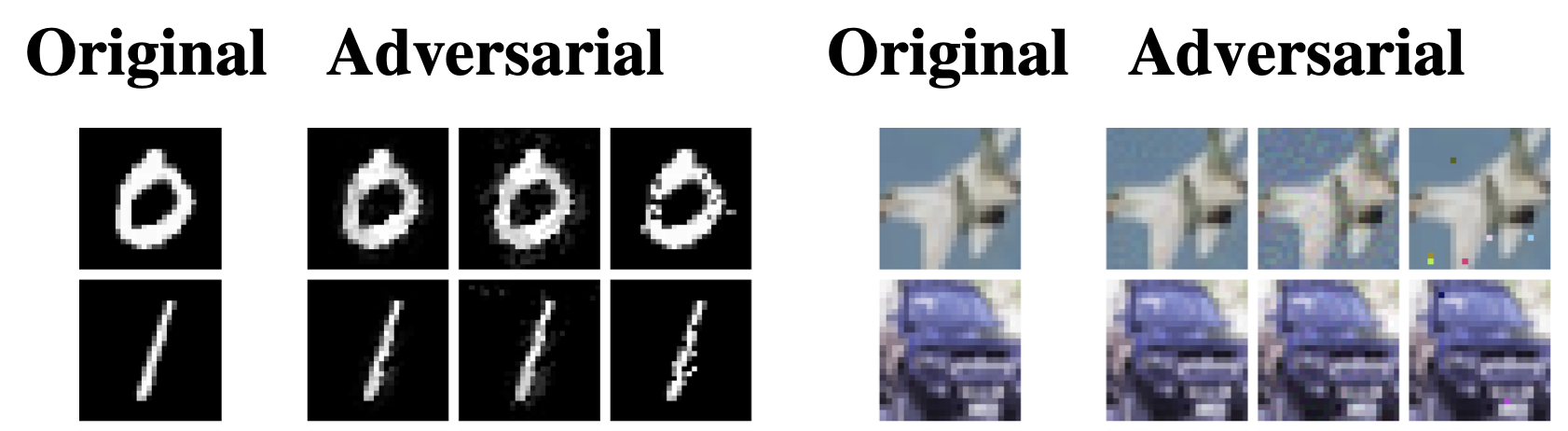
An application in data space: adversarial robustness
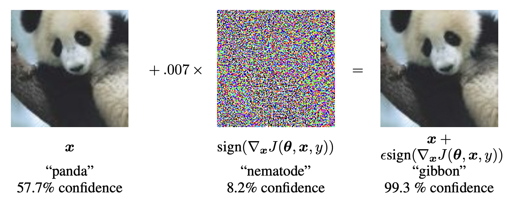
An adversarial attack perturbs a data point within the data space such that the model misclassifies it. Usually, we take \(x' = x + \delta\) while keeping the distance \(d(x, x')\) small (i.e., less than some small \(\varepsilon\)), so that the perturbation is imperceptible to humans. The choice of metric fundamentally changes what the attack looks like:- The most common attack uses the \(L_{\infty}\) norm, where \(||x-x'||_{\infty} = \max_i |x_i - x'_i| \leq \varepsilon\) means that each pixel can be perturbed by at most \(\varepsilon\). This takes advantage of the fact that a human probably won't notice a small change in any single pixel.
In 2014, Goodfellow et al. introduced the Fast Gradient Sign Method (FGSM), which creates adversarial examples that maximizes a classification model's loss (and therefore its misclassification probability). Given an input \(x\) with a true output \(y\), they calculate the gradient of the loss with respect to the input \(\nabla_x L(\theta, x, y)\) and create an adversarial sample using \(x' \gets x + \varepsilon \cdot \text{sign}(\nabla_x L(\theta, x, y))\). This method effectively perturbs each pixel in the direction that increases the loss the most, while keeping the perturbation within the \(L_{\infty}\) norm constraint.
- Using the \(L^2\) norm \(||x-x'||_2 = \sqrt{\sum_i (x_i - x'_i)^2} \leq \varepsilon\) allows for larger perturbations in some pixels, as long as the overall energy of the perturbation remains below a certain threshold, resulting in more localized changes.
The Carlini-Wagner method generates adversarial samples in the data space \(\mathbb{R}^n\)by solving the optimization problem given by \(\min ||x - x'||_2 + c f(x')\) such that \(x' \in [0,1]^n\), where \(f\) is one of many functions that encourages misclassification. For instance, given an adversarial target class \(t\), the function \(f(x') = \text{softplus} (\max \{Z(x')_i: i \neq t\} - Z(x')_t) - \ln(2)\) encourages \(x'\) to be classified as class \(t\).
- Using the \(L^1\) norm \(||x-x'||_1 = \sum_i |x_i - x'_i| \leq \varepsilon\) encourages sparse perturbations, meaning that only a few pixels are changed significantly while others remain untouched.
A model that is robust to an adversarial attack using the \(L_{\infty}\) norm may not be robust to attacks using the \(L^2\) or \(L^1\) norms, and vice versa. In high dimensions, a ball defined by the \(L^2\) norm and a ball defined by the \(L^1\) norm have almost no overlap – the topology defined by each metric gives an entirely different of what "near" means. Understanding the choice of metric is necessary to design effective adversarial defenses and evaluate model robustness.
An application in function space: mode connectivity
In any number of dimensions, two trained neural networks with different parameters \(\theta_1\) and \(\theta_2\) can have similar functional forms. Expressed in distance, we can counterintuitively see a large \(||\theta_1 - \theta_2||_{\text{param}}\) alongside a small \(||f(\theta_1) - f(\theta_2)||_{\text{function}}\). Our sinusoidal example \(f(x; A, \omega) = A \sin(\omega x)\) makes this clear: for parameter values \((A, \omega) = (1,2)\) and \((-1, -2)\), the functional distance \(||1 \cdot \sin(2 \cdot x) - (-1) \cdot \sin((-2) \cdot x)||\) is zero, even though the parameter distance \(\sqrt{(1-(-1))^2 + (2-(-2))^2} \approx 4.47\) is quite large.This is partly because the realization function \(\Phi: \Theta \to \mathcal{F}\) is highly non-injective: many different parameter values, sometimes infinitely many, could map to the same or similar functions. This is a feature of overparameterization, but introducing and tracking a metric in function space, as well as in parameter space, has been shown to improve our understanding of model behavior.
An application in probability space: GANs
A generative adversarial network (GAN) consists of two networks: a generator \(G\) that creates fake data from random noise, and a discriminator \(D\) that tries to distinguish between real and fake data. The goal of the generator is to produce data that is indistinguishable from real data, while the discriminator aims to correctly classify real and fake data. They used to work by matching a generated distribution \(p_g\) to a real distribution \(p_r\) using the Jensen-Shannon divergence, given by \[ D_{JS}(p_g || p_r) = \frac{1}{2}[D_{KL}(p_g||m) + D_{KL}(p_r || m)], \] where \(m = \frac{1}{2}(p_g + p_r)\) and \(D_{KL}\) is the Kullback-Leibler divergence, itself a measure of distance between probability distributions given by \[ D_{KL}(P||Q) = \sum_{x \in X} P(x) \log \frac{P(x)}{Q(x)}. \]However, the JS divergence is not a metric: it violates both symmetry and the triangle inequality. Moreover, if the distributions have disjoint support (i.e., no overlap), \(D_{JS} = \log(2)\) everywhere.
Arjovsky et al. proposed to use the Wasserstein distance, a proper metric on the space of probability distributions given by \[W(p_g, p_r) = \inf_{\gamma \in \Gamma(p_g, p_r)} \mathbb{E}_{(x,y) \sim \gamma} [d(x,y)],\]
where \(\Gamma(p_g, p_r)\) is the set of all joint distributions \(\gamma(x,y)\) whose marginals are \(p_g\) and \(p_r\), respectively, and \(d(x,y)\) is a distance metric on the underlying data space. The Wasserstein distance measures the minimum "cost" of transporting mass to transform one distribution into another, providing meaningful measure of distance between distributions, even when they have disjoint support.
The measure
The measure is a distinct and more theoretical concept than the metric, though the two are related. Broadly, a measure is a function that measures the size or volume of a given set. More formally, a measure \(\mu\) on a set \(S\) is a function that assigns a non-negative real number \(\mu(A)\) to each subset \(A\) of \(S\), satisfying some familiar properties:
- Non-negativity: \(\mu(A) \geq 0\) for any subset \(A\) of \(S\).
- Null empty set: \(\mu(\emptyset) = 0\).
- Countable additivity: For any countable collection of disjoint subsets \(A_1, A_2, \ldots\) of \(S\), \(\mu\left(\bigcup_{i=1}^{\infty} A_i\right) = \sum_{i=1}^{\infty} \mu(A_i)\).
Often it's sufficient to prove that things won't happen ("almost certainly") by showing that the set on which they could happen has measure zero. In the neural tangent kernel, for instance, the set of initializations that fail to converge to a deterministic limiting kernel has measure zero, so a given initialization will almost certainly converge.
Measures come up often in integration. The form of integration we're used to seeing, \(\int_X f(x) dx\), is a special case of the Lebesgue integral with respect to a measure, whose general form is the uncanny-looking \(\int_X f d \mu\), where \(\mu\) is a measure on \(X\), and \(dx\) is shorthand for integration with respect to the Lebesgue measure on \(\mathbb{R}^n\). Using this generalization, the standard integral \(\int_X f(x) dx\) and the summation \(\sum_{x \in X} f(x)\) can both be expressed as Lebesgue integrals with respect to different measures: the Lebesgue measure for the integral, and the counting measure for the summation.
This allows us to generalize some important operations. In evaluating empirical risk, for instance, our data gives a so-called empirical measure \(\mu_N = \frac{1}{N} \sum_{i=1}^N \delta_{x_i}\), so that empirical risk looks like integration: \( \mathcal{L}_{\text{emp}} = \int \ell [f_{\theta}(x), y] dy \).Conclusion
Understanding the distinction between metrics and measures provides a tool for reasoning about machine learning systems. Metrics help us navigate optimization landscapes and evaluate model behavior, while measures give us the theoretical foundations for integration and probabilistic reasoning. We can design much better, more rigorous algorithms by carefully choosing and understanding our measurement frameworks.
© Jamie Mahowald